 foxxcyber/docs
Tables, formatting and charts
Style tables in documents, insert charts from typed data or a spreadsheet's cells, and format spreadsheets: quick styles, Format as Table, conditional formatting, freezing and charts.
The document and spreadsheet editors in the Document Library can style tables, draw charts and format data, much as Word and Excel do. Everything is saved as ordinary Word and Excel formatting, so the files look the same when opened in Word, Excel or LibreOffice.
Tables in documents
Insert a table with the table button in the toolbar, then click in it. The Table format button next to it opens the table menu.
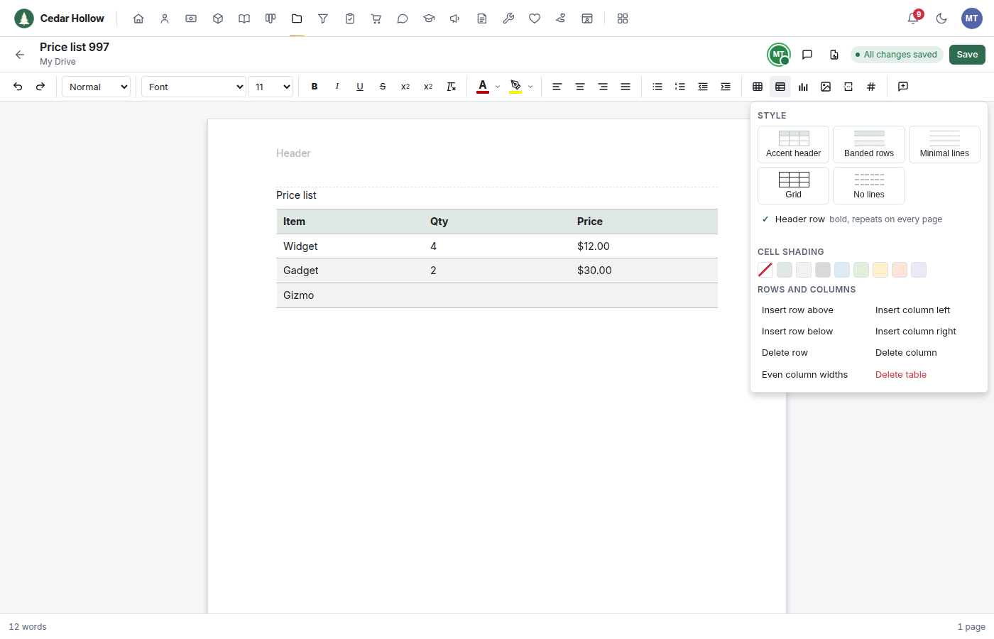
- Style restyles the whole table in your organization's colour (Settings → Organization). Accent header tints the header row, Banded rows shades every other row, Minimal lines keeps only the lines between rows, and No lines is for layout tables.
- Header row makes the first row bold and repeats it at the top of every page the table runs onto.
- Cell shading colours the cell you are in.
- Rows and columns inserts or deletes rows and columns, evens out the column widths, or deletes the table. A banded table stays banded as rows come and go.
Charts in documents
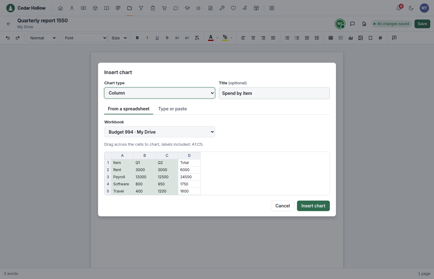
- Put the cursor where the chart goes and click the chart button.
- Choose the Chart type (Column, Bar, Line, Area or Pie) and an optional Title.
- Give it the data:
- From a spreadsheet: choose a Workbook from your libraries (and a Sheet), then drag across the cells to chart, labels included.
- Type or paste: type the values, or paste cells copied from a spreadsheet. The first row names the series; the first column holds the categories.
- Click Insert chart, then Save.
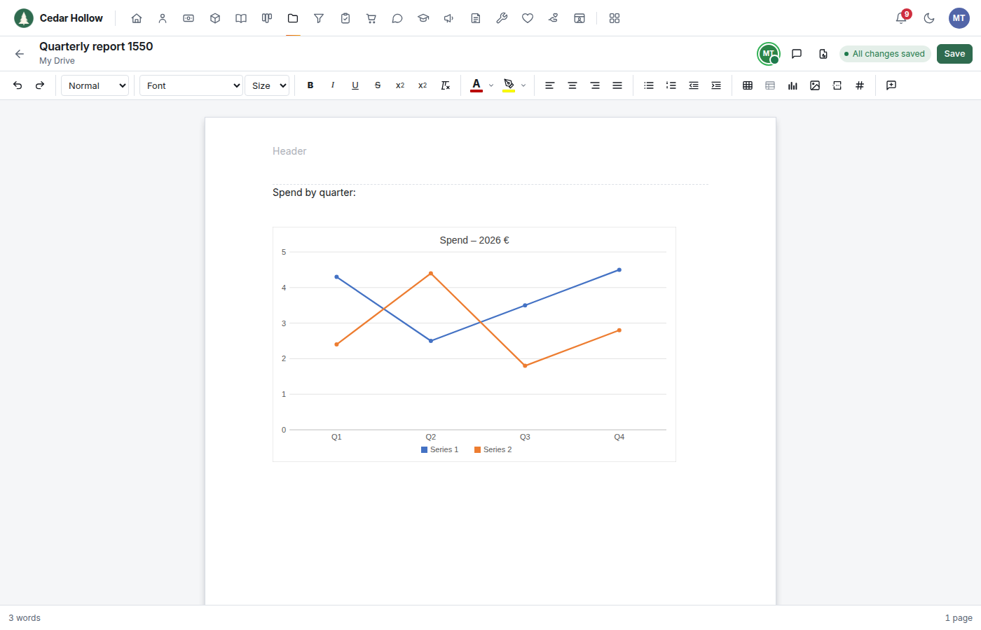
The chart is saved as a real Word chart with its data inside the
document, so Edit Data in Word opens it. The data is copied when you
insert the chart: changing the workbook later doesn't change the chart.
Charts appear in the preview and in the PDF too. Charts can be inserted
into Word (.docx) documents.
Formatting spreadsheets
Select the cells first; then:
- Quick style formats the selection as a table with the document styles above (Accent header, Banded rows, Minimal lines, Grid, No lines) in your organization's colour.
- Size sets the font size.
- Freeze keeps the Top row, the First column, or everything above and to the left of the selected cell in view while you scroll. Unfreeze undoes it. (Excel workbooks only.)
- Number format offers Number, negatives in red, Currency,
Accounting, Percent, Scientific, Fraction, dates, times and durations,
each with an example. Custom format… takes any Excel format code
(for example
#,##0.00;[Red](#,##0.00)). A cell whose format is not in the list shows it as Custom. - Decrease decimal places and Increase decimal places (beside the number format) take one place off or add one.
- Negative numbers in a format with
[Red]show in red. - Bold, italic, colours, borders, alignment, wrapping and merging are in the toolbar as before.
Format as Table
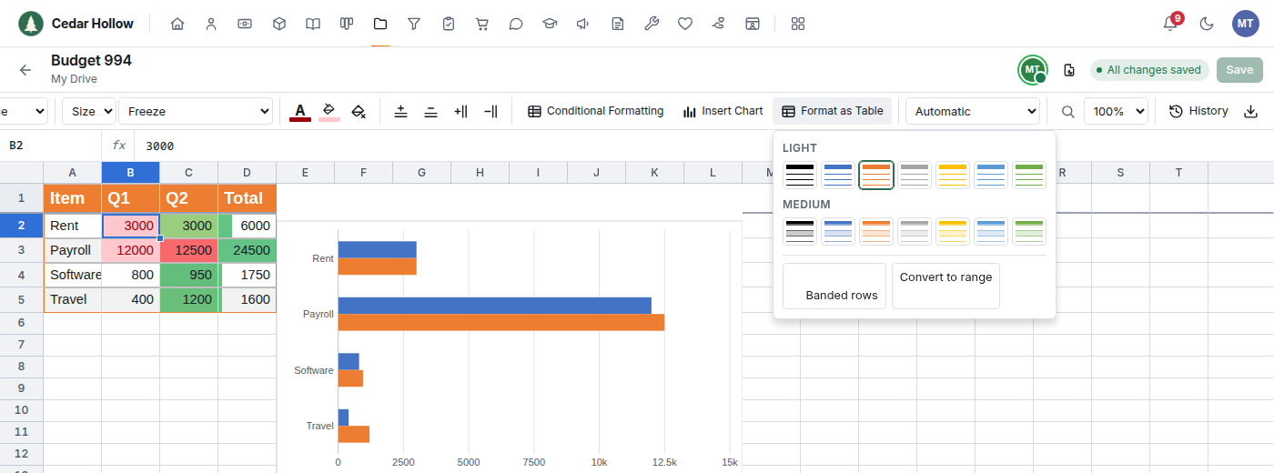
Format as Table works like Excel's: a gallery of table styles in the workbook's own colours. Over a plain selection it turns it into an Excel table in that style (the first row becomes the header row). Over a table it changes the table's style, switches Banded rows, or Convert to range.
Conditional formatting
Conditional Formatting colours cells by their values, as in Excel.
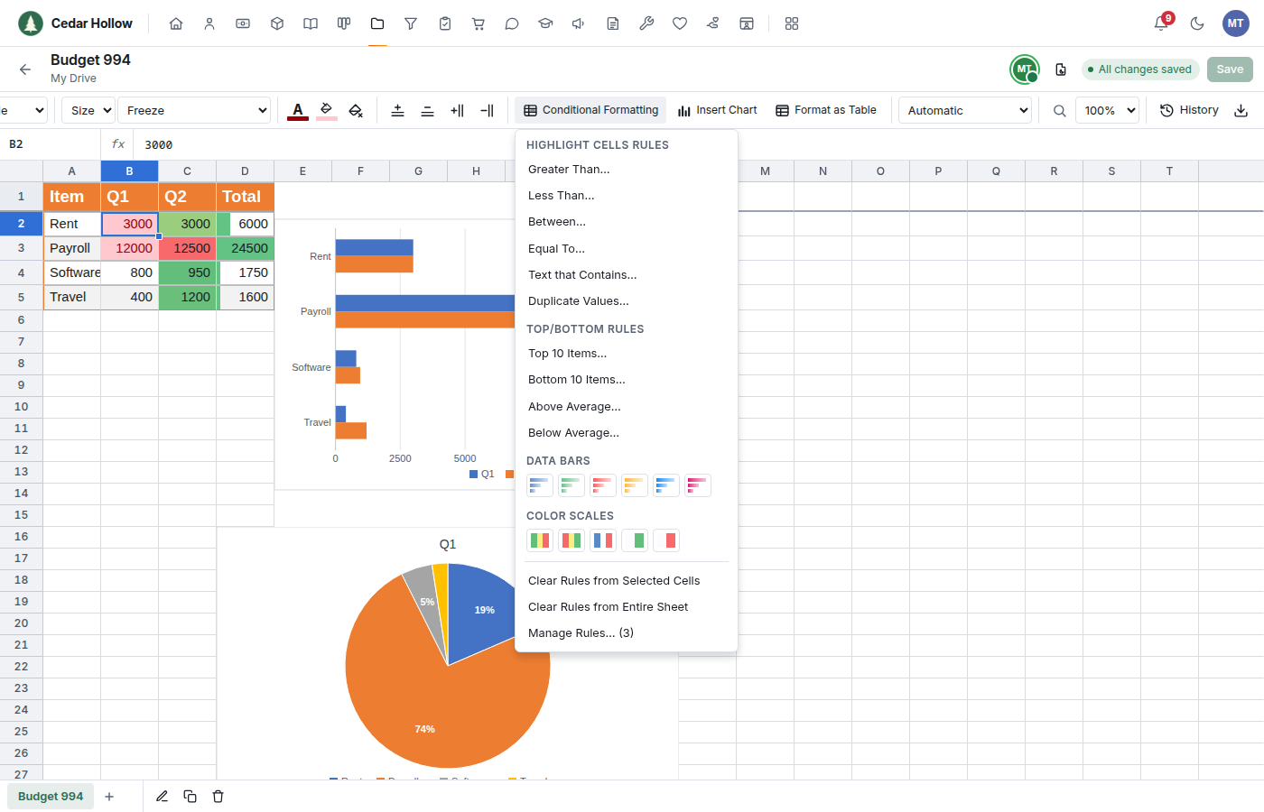
- Highlight Cells Rules: Greater Than, Less Than, Between, Equal To, Text that Contains and Duplicate Values. Each asks for the value and a format, such as Light red fill with dark red text.
- Top/Bottom Rules: the top or bottom items (or percent), and cells above or below the average.
- Data Bars draw a bar in each cell sized by its value.
- Color Scales shade the cells from low to high.
- Clear Rules removes the rules on the selected cells or the whole sheet, and Manage Rules lists every rule on the sheet to delete them.
The colours update when you save. Rules made in Excel, including ones the editor can't draw (formulas, icon sets), are kept as they are.
Charts in spreadsheets
Select the numbers with their labels and choose Insert Chart: Column, Bar, Line, Area or Pie. The top row names the series and the left column holds the categories. The chart reads the cells, so it changes when they do.
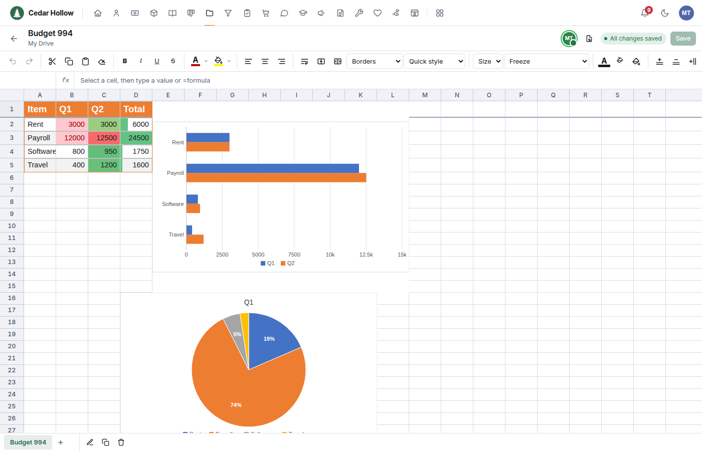
Click a chart to pick it. Drag it to move it, drag its corner to resize it, and use Chart type or the delete button that appear in the toolbar (or press Delete). Charts are saved as Excel charts, so they open in Excel and LibreOffice, and charts made in Excel show here.